Preparing your dataset: Data Cleaning and Descriptives
In this lab, you will learn how to clean up a dataset to prepare it for analyses.
Task 1. Initial cleaning of a dataset
We will use a provided dataset for this task. Note that this file is still cleaned up to some extent. When you download a completed survey from Qualtrics, it will have many additional columns that are mostly not needed for data analysis and we will not normally use them.
Q1. Download the Lab 03 Dataset.xlsx and Lab 03 Codebook.xlsx files from Learn. The first file is the dataset (note that some small modifications have been made to protect respondents’ privacy). Responses have also been coded according to the codebook file—take a few minutes to read through the codebook so you understand this dataset.
tibble [140 × 30] (S3: tbl_df/tbl/data.frame)
$ RESP_ID : chr [1:140] "Response ID" "1" "2" "3" ...
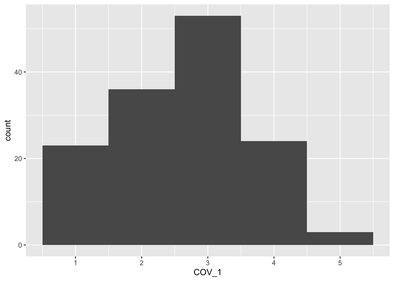
$ COV_1 : chr [1:140] "Just prior to lockdown, how worried were you about your likelihood of contracting COVID-19?" "2" "3" "2" ...
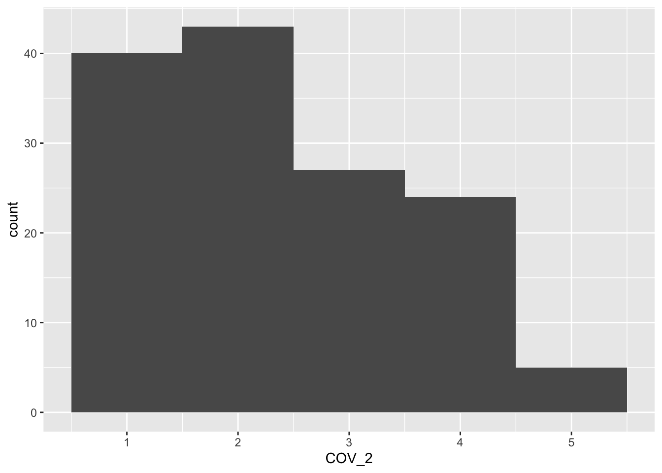
$ COV_2 : chr [1:140] "Just prior to lockdown, how worried were you about suffering serious medical complications if you contracted COVID-19?" "2" "2" "2" ...
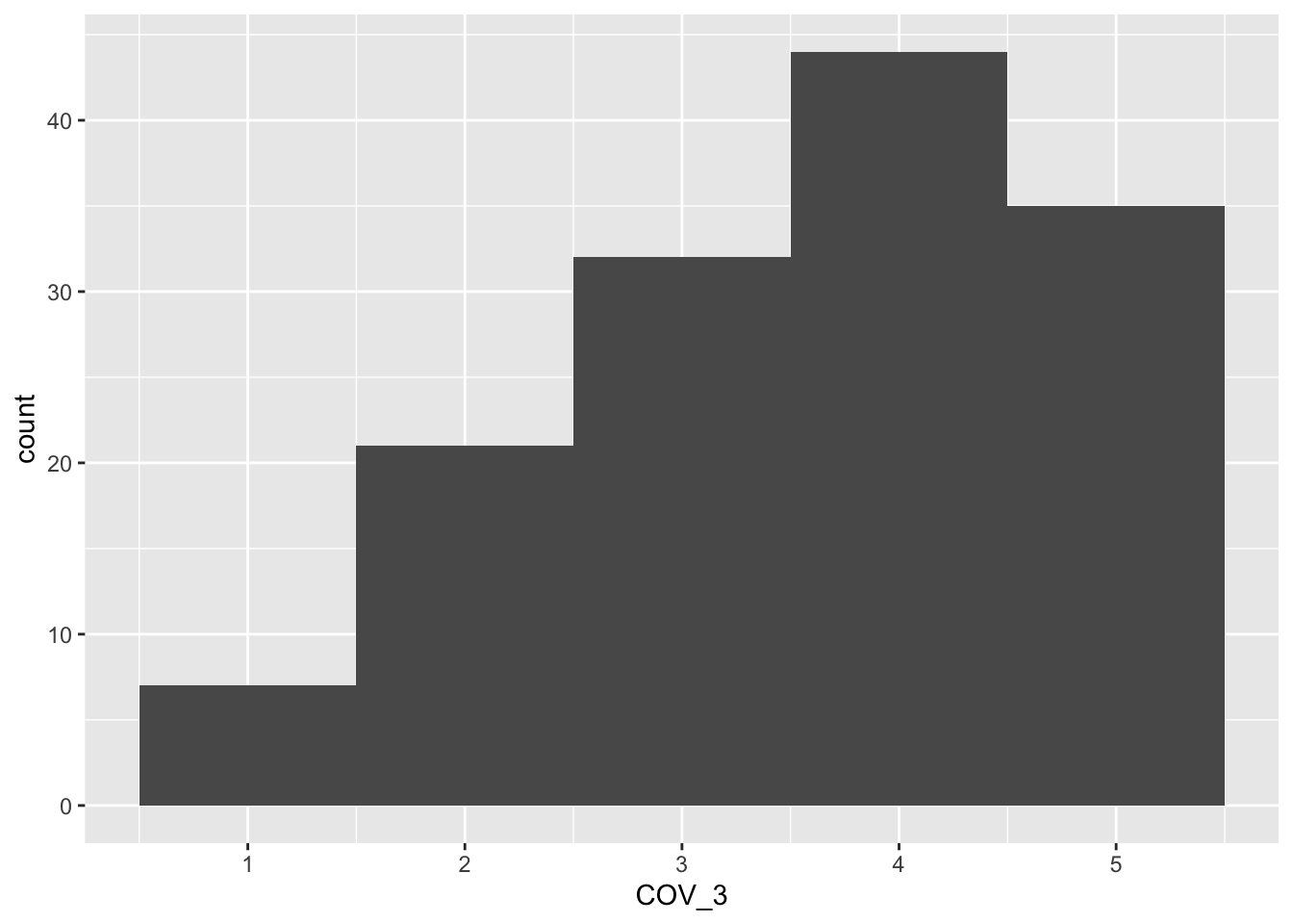
$ COV_3 : chr [1:140] "Just prior to lockdown, how worried were you about passing COVID-19 on to someone else if you contracted it?" "2" "3" "2" ...
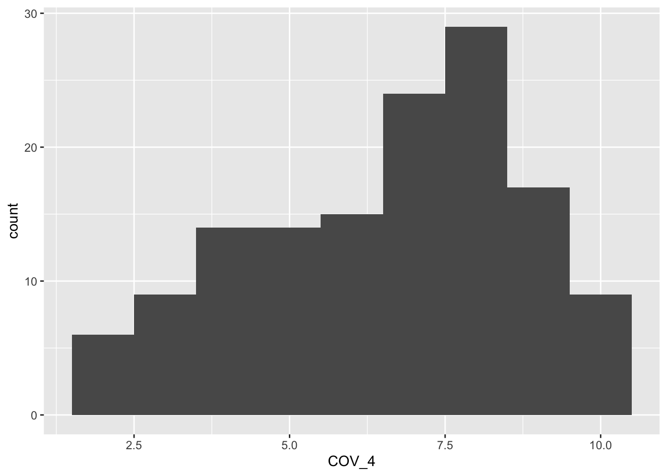
$ COV_4 : chr [1:140] "On a scale of 1-10, how well would you say you coped overall during lockdown?" "8.3000000000000007" "9.1999999999999993" "5.7" ...
$ COV_9a : chr [1:140] "Ease of access: Academic support" "3" "3" "5" ...
$ COV_9b : chr [1:140] "Ease of access: Financial help" NA NA "5" ...
$ COV_9c : chr [1:140] "Ease of access: Health services" "4" "3" "4" ...
$ COV_9d : chr [1:140] "Ease of access: Mental health services" NA NA "4" ...
$ COV_9e : chr [1:140] "Ease of access: Other" NA NA NA ...
$ COV_10 : chr [1:140] "How do you feel the pandemic impacted your academic performance in Semester 1?" "4" "3" "4" ...
$ FIN_1_1 : chr [1:140] "I constantly worry about my financial situation" "3" "3" "5" ...
$ FIN_1_2 : chr [1:140] "I try not to think about how much debt I am in" "4" "6" "2" ...
$ FIN_1_3 : chr [1:140] "My income is sufficient to meet my needs" "5" "6" "3" ...
$ FIN_1_4 : chr [1:140] "I think my financial position has a negative effect on my social life" "4" "5" "5" ...
$ FIN_1_5 : chr [1:140] "I think my financial position has a negative effect on my study" "3" "2" "6" ...
$ FIN_1_6 : chr [1:140] "Not meeting my weekly financial demands is constantly on my mind" "4" "3" "5" ...
$ FIN_1_7 : chr [1:140] "Worrying about money affects my daily mood" "4" "5" "5" ...
$ FIN_1_8 : chr [1:140] "I feel like I don’t have enough money to do the things I enjoy" "4" "5" "5" ...
$ FIN_2_1 : chr [1:140] "I find myself stressing about upcoming payments" "5" "2" "5" ...
$ FIN_2_2 : chr [1:140] "I feel stressed when I receive my bills" "4" "6" "5" ...
$ FIN_2_3 : chr [1:140] "I am often concerned I will not have enough funds to make necessary purchases" "5" "2" "4" ...
$ FIN_2_4 : chr [1:140] "I spend all my money on living costs" "4" "1" "3" ...
$ FIN_2_5 : chr [1:140] "I regularly miss out on social occasions due to finances" "5" "4" "3" ...
$ FIN_2_6 : chr [1:140] "I compromise my well-being due to my financial situation" "4" "4" "4" ...
$ FIN_2_7 : chr [1:140] "I am able to easily balance my finances with my social life" "5" "3" "4" ...
$ FIN_2_8 : chr [1:140] "Financial stress restricts my social life" "4" "5" "5" ...
$ FIN_2_9 : chr [1:140] "I avoid interactions that involve money" "4" "6" "5" ...
$ Age_coded: chr [1:140] "Age" "19-24" "19-24" "19-24" ...
$ Gender : chr [1:140] "What gender do you identify with?" "Male" "Female" "Female" ...
Q2. Open the dataset file with R. Discuss with your peer why you should delete the first row.
df <- df[-c(1), ]
Q3. Use your codebook to determine if R has the correct measurement type (nominal, ordinal, or continuous) and data type (integer, decimal, text) and make changes if they are not correct.
We can see that all continuous measures (cloums 2:27) that are supposed to be numeric, are string (character). We need to change them to numeric first.
Now we will look at another variable more deeply and figure out if their distribution is normal. This is important as we go into inferential statistics, we are required to check all variables for the assumption of normality (amongst other assumption tests) before we run our analyses.
Q3. Calculate Mean, Standard deviation, Skewness, and Shapiro-Wilk.
psych::describe(df$COV_4)
   vars   n mean   sd median trimmed  mad min max range  skew kurtosis   se
X1    1 137 6.58 2.19    7.1    6.68 2.22 1.8  10   8.2 -0.41    -0.84 0.19
shapiro.test(df$COV_4)
    Shapiro-Wilk normality test

data:  df$COV_4
W = 0.94971, p-value = 6.908e-05
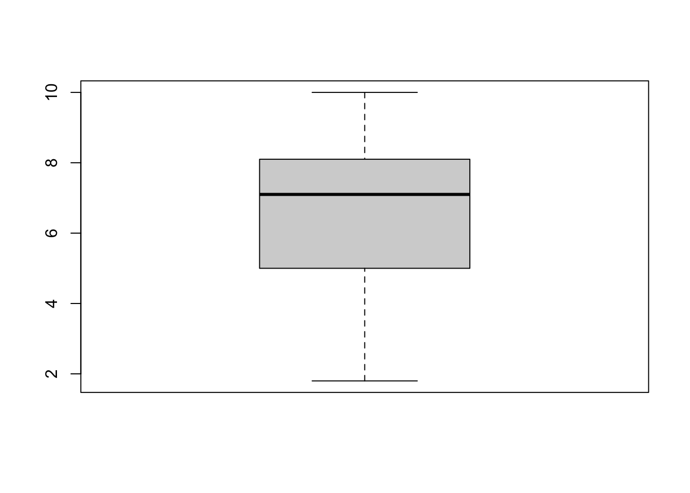
Q4. What do these statistics, alongside the graphs, tell us about the distribution of responses to this question?
Where is it centred?
Is it normal?
Is it skewed?
Task 3. Testing hypotheses.
We now want to test two directionality hypotheses to have a basic understanding of how our variables relate to each other. This is a step called exploratory data analysis.
Firstly, we want to know the directionality of the relationship between how well students coped during lockdown ‘COV_4’ and their impression of how the pandemic has impacted their academic performance ‘COV_10’.
Q1. Calculate the correlation between COV_4 and COV_10. using ‘Kendall’s tau-b’. NOTE: We use this statistic because COV_10 is technically ordinal, rather than scale. You use the same guidelines as Pearson’s r to assess strength i.e. 0.1, 0.3, and 0.5 for weak, moderate, and strong, respectively.
    Kendall's rank correlation tau

data:  df$COV_4 and df$COV_10
z = -4.4807, p-value = 7.441e-06
alternative hypothesis: true tau is not equal to 0
sample estimates:
       tau
-0.3185941
Q2. What do the correlation coefficient tell us about the relationship between how well someone thought they coped overall during lockdown (COV_4) and how they feel the pandemic affected their academic performance (COV_10). Make note of: a. The direction of the correlation. HINT: Refer to the codebook for how the response scales are for both variables. b. The strength of the correlation. c. Whether the correlation is statistically significant.
Q3. Do you think having a worse experience of lockdown overall tended to result in poorer academic performance, or did poorer academic performance result in a worse experience of lockdown overall? What do the correlational data tell us about which is more likely?
Q4. We want to know the directionality of the relationship between how well students coped during lockdown ‘COV_4’ and their financial stress. Calculate correlation between COV_4 and the financial stress composite variable that you created, using ‘Pearson’ correlation.
    Pearson's product-moment correlation

data:  df$COV_4 and df$SFSS_A
t = -0.56441, df = 135, p-value = 0.5734
alternative hypothesis: true correlation is not equal to 0
95 percent confidence interval:
 -0.2144895  0.1201740
sample estimates:
       cor
-0.0485194
Q5.. What does the correlation coefficient tell us about the relationship between how well someone thought they coped overall during lockdown (COV_4) and their financial stress?