In this lab, you will be conducting t-tests with Jamovi and practice reporting results in APA-style format. As you heard in the lectures, we will always encounter violations of assumptions when dealing with real-life data. This lab exercise has many such instances and we will practice how to choose from non-parametric tests when assumptions are violated. We will also be reporting effect sizes. Note the interpretation guidelines for “Cohen’s d” and for “Rank biserial correlation” (0.2 = ‘small’; 0.5 = ‘medium’; 0.8 = ‘large’). This lab is important because you will learn how to choose a statistical analysis plan based on the research question, how variables were measured, and the characteristics of the dataset. These are important skills that will be assessed in your Lab Report.
Learning outcomes
At the end of this lab you will be able to: 1) Conduct and interpret a t-test with Jamovi. 2) Check assumptions and decide the corresponding non-parametric tests when needed. 3) Report findings in APA-style.
Task 1: Living with partner and getting on
Did people who lived with their partner get on better or worse with their cohabitant(s) over lockdown than people who did not live with a partner?
Q1. Open the dataset that we used in one of the previous labs (you can download the ‘Lab 5 dataset.xlsx’ file from the lab section on Learn). Read through the codebook to get an understanding of the survey questions in the dataset. Let’s have a look at the structure too.
tibble [140 × 14] (S3: tbl_df/tbl/data.frame)
 $ RESP_ID  : chr [1:140] "Response ID" "1" "2" "3" ...
 $ COV_5a   : chr [1:140] "Lived with: My partner" "0" "1" "1" ...
 $ COV_5b   : chr [1:140] "Lived with: My child(ren)" "0" "0" "0" ...
 $ COV_5c   : chr [1:140] "Lived with: My parent(s)" "1" "1" "1" ...
 $ COV_5d   : chr [1:140] "Lived with: My sibling(s)" "0" "0" "0" ...
 $ COV_5e   : chr [1:140] "Lived with: Other people related to me (eg extended family)" "0" "1" "0" ...
 $ COV_5f   : chr [1:140] "Lived with: Other people not related to me (eg flatmates)" "0" "0" "1" ...
 $ COV_5g   : chr [1:140] "Lived with: hall of residence or hostel" "0" "0" "0" ...
 $ COV_5h   : chr [1:140] "Lived with: I lived alone" "0" "0" "0" ...
 $ COV_6    : chr [1:140] "Were your living arrangements during lockdown (in terms of who you lived with):" "Different" "Different" "Different" ...
 $ COV_7    : chr [1:140] "Thinking about the people you lived with during lockdown, on a scale of 1-10, how well do you feel you got alon"| __truncated__ "9.1999999999999993" "7.1" "4" ...
 $ COV_15   : chr [1:140] "In general, how strongly do you agree or disagree with the government's decision to implement Level 4 lockdown in New Zealand?" "5" "5" "5" ...
 $ Age_coded: chr [1:140] "Age group" "19-24" "19-24" "19-24" ...
 $ Gender   : chr [1:140] "What gender do you identify with?" "Male" "Female" "Female" ...
Q2. First we are going to investigate whether people who lived with their partner get on better or worse with their cohabitant(s) over lockdown than people who did not live with a partner. From your understanding of the codebook, what is your independent variable and what is your dependent variable?
Q3. What type of analysis is appropriate given these variables?
HINT: Use your statistics decision-making tree and your codebook to help you with this question.
Better to rename our variables and also make sure the variable types are appropriate for analysis.
Generally, we would go for a t-test for independent means.
t.test(gettingOn ~ livedPartner, alt ="two.sided", conf =0.95, var.eq = T, data = df)
    Two Sample t-test

data:  gettingOn by livedPartner
t = -2.2637, df = 134, p-value = 0.0252
alternative hypothesis: true difference in means between group 0 and group 1 is not equal to 0
95 percent confidence interval:
 -1.5461757 -0.1042031
sample estimates:
mean in group 0 mean in group 1
       7.547727        8.372917
Q4. Test the assumptions of homogeneity and normality. What is the conclusion of your assumption tests? What does this mean for hypothesis testing?
NOTE: Violation of normality can be better understood graphically—if you run descriptives and create histograms graphs of your study variables, you can see more easily that the curve is not normal.
Let’s look at normality first.
shapiro.test (df$gettingOn)
    Shapiro-Wilk normality test

data:  df$gettingOn
W = 0.87295, p-value = 1.978e-09
Now, to homogneity of variance.
car::leveneTest(gettingOn ~ livedPartner, df)
Warning in leveneTest.default(y = y, group = group, ...): group coerced to
factor.
Levene's Test for Homogeneity of Variance (center = median)
       Df F value Pr(>F)
group   1  1.9741 0.1623
      134
As we can see, the assumption of normality is violated. So, let’s conduct a Mann-Whitney U test instead.
wilcox.test(gettingOn ~ livedPartner, df)
    Wilcoxon rank sum test with continuity correction

data:  gettingOn by livedPartner
W = 1547, p-value = 0.009829
alternative hypothesis: true location shift is not equal to 0
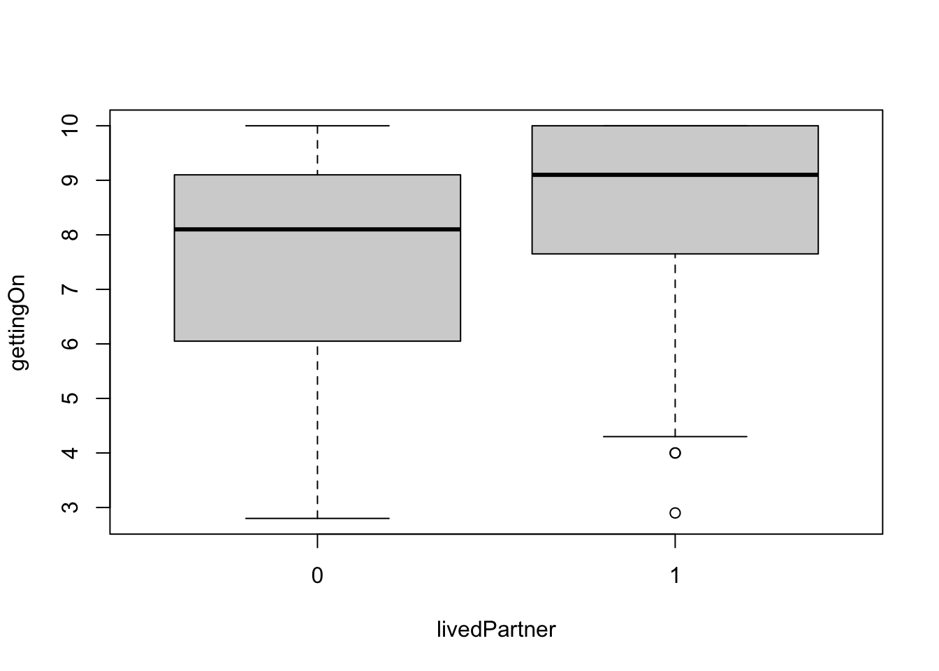
Q5. In the ‘Additional statistics’, select ‘Effect size’, ‘Descriptives’, and ‘Descriptives plots’. Report your NHST results and interpret your findings:
Mean or Median scores for each group on the dependent variable
The appropriate statistic (t or otherwise)
Significance (or otherwise) of the test
Effect size
NOTE: A measure of effect size for a t-test is the Cohen’s d. A measure of effect size for a non-parametric test is the rank biserial correlation.
Let’s do the rest of it with jamovi. The outcome is a bit different because they might be using different packages.
 INDEPENDENT SAMPLES T-TEST

 Independent Samples T-Test
 ─────────────────────────────────────────────────────────────────────────────────────────────────────
                                  Statistic    p                                         Effect Size
 ─────────────────────────────────────────────────────────────────────────────────────────────────────
   gettingOn    Mann-Whitney U     1547.000    0.0098285    Rank biserial correlation      0.2675189
 ─────────────────────────────────────────────────────────────────────────────────────────────────────


 ASSUMPTIONS

 Normality Test (Shapiro-Wilk)
 ────────────────────────────────────────
                W            p
 ────────────────────────────────────────
   gettingOn    0.8915312    < .0000001
 ────────────────────────────────────────
   Note. A low p-value suggests a
   violation of the assumption of
   normality


 Homogeneity of Variances Test (Levene's)
 ───────────────────────────────────────────────────
                F           df    df2    p
 ───────────────────────────────────────────────────
   gettingOn    2.634183     1    134    0.1069362
 ───────────────────────────────────────────────────
   Note. A low p-value suggests a violation of
   the assumption of equal variances


 Group Descriptives
 ─────────────────────────────────────────────────────────────────────────────
                Group    N     Mean        Median      SD          SE
 ─────────────────────────────────────────────────────────────────────────────
   gettingOn    0        88    7.547727    8.100000    2.113230    0.2252711
                1        48    8.372917    9.100000    1.871027    0.2700594
 ─────────────────────────────────────────────────────────────────────────────
Task 2: Change in living arrnagement and getting on
Did people whose living arrangements changed just prior to lockdown get on better or worse with their cohabitant(s) than those whose living arrangements stayed the same?
Q6. Now we are going to investigate whether people whose living arrangements changed just prior to lockdown get on better or worse with their cohabitant(s) than those whose living arrangements stayed the same. From your understanding of the codebook, what is your independent variable and what is your dependent variable?
Q7. What type of analysis is appropriate given these variables?
t.test(gettingOn ~ changedCond, alt ="two.sided", conf =0.95, var.eq = T, data = df)
    Two Sample t-test

data:  gettingOn by changedCond
t = -0.28567, df = 133, p-value = 0.7756
alternative hypothesis: true difference in means between group Different and group Same is not equal to 0
95 percent confidence interval:
 -0.8318547  0.6218934
sample estimates:
mean in group Different      mean in group Same
               7.806383                7.911364
Q8. In ‘Assumption checks’, select ‘Homogeneity test’ and ‘Normality test’. What is the conclusion of your assumption tests? What does this mean for hypothesis testing?
Q9. In the ‘Additional statistics’, select ‘Effect size’, ‘Descriptives’, and ‘Descriptives plots’. Report your NHST results and interpret your findings:
Mean or Median scores for each group on the dependent variable
The appropriate statistic (t or otherwise)
Significance (or otherwise) of the test
Effect size
Assumptions: We already know that normality is violated.
shapiro.test (df$gettingOn)
    Shapiro-Wilk normality test

data:  df$gettingOn
W = 0.87295, p-value = 1.978e-09
Homogeneity of variance
car::leveneTest(gettingOn ~ changedCond, df)
Levene's Test for Homogeneity of Variance (center = median)
       Df F value Pr(>F)
group   1  0.9051 0.3431
      133
Mann-Whitney U test
wilcox.test(gettingOn ~ changedCond, df)
    Wilcoxon rank sum test with continuity correction

data:  gettingOn by changedCond
W = 1917.5, p-value = 0.4865
alternative hypothesis: true location shift is not equal to 0
 INDEPENDENT SAMPLES T-TEST

 Independent Samples T-Test
 ─────────────────────────────────────────────────────────────────────────────────────────────────────
                                  Statistic    p                                         Effect Size
 ─────────────────────────────────────────────────────────────────────────────────────────────────────
   gettingOn    Mann-Whitney U     1547.000    0.0098285    Rank biserial correlation      0.2675189
 ─────────────────────────────────────────────────────────────────────────────────────────────────────


 ASSUMPTIONS

 Normality Test (Shapiro-Wilk)
 ────────────────────────────────────────
                W            p
 ────────────────────────────────────────
   gettingOn    0.8915312    < .0000001
 ────────────────────────────────────────
   Note. A low p-value suggests a
   violation of the assumption of
   normality


 Homogeneity of Variances Test (Levene's)
 ───────────────────────────────────────────────────
                F           df    df2    p
 ───────────────────────────────────────────────────
   gettingOn    2.634183     1    134    0.1069362
 ───────────────────────────────────────────────────
   Note. A low p-value suggests a violation of
   the assumption of equal variances


 Group Descriptives
 ─────────────────────────────────────────────────────────────────────────────
                Group    N     Mean        Median      SD          SE
 ─────────────────────────────────────────────────────────────────────────────
   gettingOn    0        88    7.547727    8.100000    2.113230    0.2252711
                1        48    8.372917    9.100000    1.871027    0.2700594
 ─────────────────────────────────────────────────────────────────────────────
Task 3: Male and female vs. govt decision
Did males and females differ with respect to their level of agreement with the government’s decision to implement the lockdown?
Q10. Now we’re going to see whether males and females differed with respect to their level of agreement with the government’s decision to implement the lockdown. From your understanding of the codebook, what is your independent variable and what is your dependent variable?
Q11. What type of analysis is appropriate given these variables?
t.test(govDecision ~ Gender, alt ="two.sided", conf =0.95, var.eq = T, data = df)
    Two Sample t-test

data:  govDecision by Gender
t = 3.2589, df = 135, p-value = 0.001415
alternative hypothesis: true difference in means between group Female and group Male is not equal to 0
95 percent confidence interval:
 0.2062318 0.8429380
sample estimates:
mean in group Female   mean in group Male
            4.731481             4.206897
Q12. Assumption checks. What is the conclusion of your assumption tests? What does this mean for hypothesis testing?
Assumptions
shapiro.test (df$govDecision)
    Shapiro-Wilk normality test

data:  df$govDecision
W = 0.52955, p-value < 2.2e-16
car::leveneTest(govDecision ~ Gender, df)
Warning in leveneTest.default(y = y, group = group, ...): group coerced to
factor.
Levene's Test for Homogeneity of Variance (center = median)
       Df F value   Pr(>F)
group   1   10.62 0.001415 **
      135
---
Signif. codes:  0 '***' 0.001 '**' 0.01 '*' 0.05 '.' 0.1 ' ' 1
Mann-Whitney U test
wilcox.test(govDecision ~ Gender, df)
    Wilcoxon rank sum test with continuity correction

data:  govDecision by Gender
W = 1919, p-value = 0.01477
alternative hypothesis: true location shift is not equal to 0
Q13. In the ‘Additional statistics’, select ‘Effect size’, ‘Descriptives’, and ‘Descriptives plots’. Report your NHST results and interpret your findings:
Mean or Median scores for each group on the dependent variable
 INDEPENDENT SAMPLES T-TEST

 Independent Samples T-Test
 ───────────────────────────────────────────────────────────────────────────────────────────────────────
                                    Statistic    p                                         Effect Size
 ───────────────────────────────────────────────────────────────────────────────────────────────────────
   govDecision    Mann-Whitney U     1213.000    0.0147729    Rank biserial correlation      0.2254151
 ───────────────────────────────────────────────────────────────────────────────────────────────────────


 ASSUMPTIONS

 Normality Test (Shapiro-Wilk)
 ──────────────────────────────────────────
                  W            p
 ──────────────────────────────────────────
   govDecision    0.6755793    < .0000001
 ──────────────────────────────────────────
   Note. A low p-value suggests a
   violation of the assumption of
   normality


 Homogeneity of Variances Test (Levene's)
 ─────────────────────────────────────────────────────
                  F           df    df2    p
 ─────────────────────────────────────────────────────
   govDecision    22.29761     1    135    0.0000058
 ─────────────────────────────────────────────────────
   Note. A low p-value suggests a violation of the
   assumption of equal variances


 Group Descriptives
 ───────────────────────────────────────────────────────────────────────────────────
                  Group     N      Mean        Median      SD           SE
 ───────────────────────────────────────────────────────────────────────────────────
   govDecision    Female    108    4.731481    5.000000    0.5897327    0.05674706
                  Male       29    4.206897    5.000000     1.235756     0.2294742
 ───────────────────────────────────────────────────────────────────────────────────